Gradient Flow with Minibatching

Gradient flow is gradient descent over continous time. Thinking about it another way, gradient descent is like applying a discrete ODE solver to a gradient flow problem. Given a set of parameters \(\theta \in \mathrm{R}^d\), we minimize an objective \(h : \mathrm{R}^d \to \mathrm{R}\) according to

\[\dot{\theta} = -\eta\nabla h(\theta).\]

Where \(\eta\) is the learning rate, which we take to be constant. Let’s consider a very simple example. Given a point \(\mathbf{a}\in\mathrm{R}^d\), we set our loss to be the squared error between \(\mathbf{a}\) and our parameters \(\theta\), \(h(\theta) := \frac{1}{2}\|\mathbf{a}-\theta\|^2\). Then the gradient flow becomes,

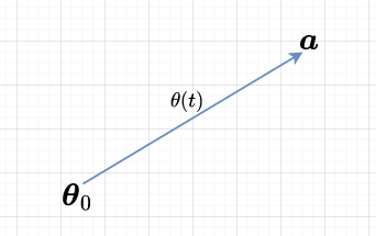
\[\dot{\theta} = \eta(\mathbf{a} - \theta).\]

Given \(\theta(0)=\boldsymbol{\theta}_0\), the solution is exactly \(\theta(t)=\mathbf{a} + (\boldsymbol{\theta}_0 - \mathbf{a})e^{-\eta t}\). Evidently, the dynamics follow a linear trajectory from \(\boldsymbol{\theta}_0\) to \(\mathbf{a}\).

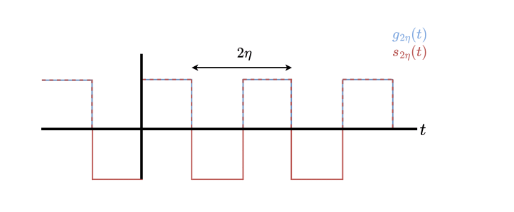
Let’s get slightly more complicated, let’s consider two datapoints: \(\mathbf{a},\mathbf{b}\). In full batch gradient descent, we compute the average loss w.r.t each datapoint before taking a gradient step. Perhaps unsurprisingly, this would result in a linear trajectory from \(\boldsymbol{\theta}_0\) to \(\frac{1}{2}(\mathbf{a} + \mathbf{b})\). In minibatch gradient descent, we break up our dataset in batches and compute the loss on a per batch basis. Typically, after a full pass through the data, we rebatch our dataset to prevent overfitting. In our case, we’ll only consider a round robin sampling between \(\mathbf{a}\) and \(\mathbf{b}\). We’ll model this as a toggeling between objectives using a square-wave with period \(2\eta\). The gradient flow is,

\[\begin{align*} \dot{\theta} &= \eta\left[g_{2\eta}(t)(\mathbf{a} - \theta) + (1-g_{2\eta}(t))(\mathbf{b} - \theta)\right] \\ &= \eta\left[g_{2\eta}(t)(\mathbf{a} - \mathbf{b}) + \mathbf{b} - \theta\right]. \end{align*}\]

where \(g_{2\eta}(t)\) is a square wave that alternates between 0 and 1 with period \(2\eta\). Note \(g_{2\eta}(t) = \frac{1}{2} + \frac{1}{2}s_{2\eta}(t)\), where \(s_{2\eta}(t)\) is a standard square wave that alternates between -1 and 1.

We can solve the above equation using the Laplace transform,

\[\begin{align*} \mathcal{L}\{\dot{\theta}\} &= \mathcal{L}\left\{\eta[\frac{\mathbf{a} + \mathbf{b}}{2} + \frac{\mathbf{a} - \mathbf{b}}{2}s_{2\eta}(t) - \theta]\right\} \\ \implies s\Theta(s) - \boldsymbol{\theta}_0 &= \frac{\eta(\mathbf{a} + \mathbf{b})}{2s} + \frac{\eta(\mathbf{a} - \mathbf{b})}{2s}\tanh(\frac{\eta s}{2}) - \eta \Theta(s) {} \\ \implies (s + \eta)\Theta(s) &= \boldsymbol{\theta}_0 + \frac{\eta(\mathbf{a} + \mathbf{b})}{2s} + \frac{\eta(\mathbf{a} - \mathbf{b})}{2s}\tanh(\frac{\eta s}{2}) \\ \implies \Theta(s) &= \frac{\boldsymbol{\theta}_0}{s+\eta} + \frac{\eta(\mathbf{a} + \mathbf{b})}{2s(s+\eta)} + \frac{\eta(\mathbf{a} - \mathbf{b})}{2s(s+\eta)}\tanh(\frac{\eta s}{2}) \\ \implies \theta(t) &= \frac{\mathbf{a} + \mathbf{b}}{2} + (\boldsymbol{\theta}_0 - \frac{\mathbf{a} + \mathbf{b}}{2})e^{-\eta t} + \frac{\mathbf{a} - \mathbf{b}}{2}\mathcal{L}^{-1}\left\{\frac{\eta}{s(s+\eta)}\tanh(\frac{\eta s}{2})\right\}. \\ \end{align*}\]

Where used the fact that \(\mathcal{L}\{s_{2\eta}(t)\}=\frac{1}{s}\tanh{\frac{\eta s}{2}}\). We can further reduce the last term to,

\[\begin{align*} \mathcal{L}^{-1}\left\{\frac{\eta}{s(s+\eta)}\tanh(\frac{\eta s}{2})\right\} &= \mathcal{L}^{-1}\left\{\left(\frac{1}{s} - \frac{1}{s+\eta}\right)\tanh(\frac{\eta s}{2})\right\} \\ &= s_{2\eta}(t) - \mathcal{L}^{-1}\left\{\frac{1}{s+\eta}\tanh(\frac{\eta s}{2})\right\} \\ &= s_{2\eta}(t) - \mathcal{L}^{-1}\left\{\frac{1}{s+\eta}\sum_{k=0}^{\infty}{e^{-2 k \eta s}-2e^{- (2k+1) \eta s}+e^{- 2(k+1) \eta s}}\right\} \\ &= s_{2\eta}(t) - \sum_{k=0}^{\infty}\left[ e^{-\eta(t-2k\eta)}u(t-2k\eta) - 2e^{-\eta(t-(2k+1)\eta)}u(t-(2k+1)\eta) + e^{-\eta(t-2(k+1)\eta)}u(t-2(k+1)\eta) \right] \\ &= s_{2\eta}(t) - e^{-\eta t}\left[\sum_{k=0}^{\infty}e^{2k\eta^2}u(t-2k\eta) - 2\sum_{k=0}^{\infty}e^{(2k+1)\eta^2}u(t-(2k+1)\eta) + \sum_{k=0}^{\infty}e^{2(k+1)\eta^2}u(t-2(k+1)\eta) \right] \\ &= s_{2\eta}(t) - e^{-\eta t}\left[ \frac{1-e^{2\eta^2(\lfloor t/2\eta \rfloor + 1)}}{1-e^{2\eta^2}} -2e^{\eta^2}\frac{1-e^{2\eta^2(\lfloor (t-\eta)/2\eta \rfloor + 1)}}{1-e^{2\eta^2}} + e^{2\eta^2}\frac{1-e^{2\eta^2(\lfloor (t-2\eta)/2\eta \rfloor + 1)}}{1-e^{2\eta^2}}\right] \\ &= s_{2\eta}(t) - \frac{e^{-\eta t}}{1-e^{2\eta^2}}\left[ 1-e^{2\eta^2(\lfloor t/2\eta \rfloor + 1)} -2e^{\eta^2}(1-e^{2\eta^2(\lfloor (t-\eta)/2\eta \rfloor + 1)}) + e^{2\eta^2}(1-e^{2\eta^2(\lfloor (t-2\eta)/2\eta \rfloor + 1)})\right]. \\ \end{align*}\]

Where \(u(t)\) is the Heaviside function (0 for t < 0, and 1 otherwise). And Voilà we’re done! Although this expression is somewhat unweildy. Let’s try to unpack what it’s saying. When \(0 \leq t<\eta\), the early dynamics should exactly match the linear dynamics towards \(\mathbf{a}\). Indeed, the last two terms are exactly zero leaving \(s_{2\eta}(t) - e^{-\eta t}\), so the full expression simplifies to

\[\frac{\mathbf{a} + \mathbf{b}}{2} + (\boldsymbol{\theta}_0 - \frac{\mathbf{a} + \mathbf{b}}{2})e^{-\eta t} + \frac{\mathbf{a} - \mathbf{b}}{2}s_{2\eta}(t) - \frac{\mathbf{a} - \mathbf{b}}{2}e^{-\eta t} = \mathbf{a} + (\boldsymbol{\theta}_0 - \mathbf{a})e^{-\eta t}.\]

In terminal dynamics, when \(t>>1\), the effect of the constant terms diminishes when multiplied by \(e^{-\eta t}\). We can simplify the term considerably:

\[\begin{align*} & \frac{e^{-\eta t}}{1-e^{2\eta^2}}\left[ 1-e^{2\eta^2(\lfloor t/2\eta \rfloor + 1)} -2e^{\eta^2}(1-e^{2\eta^2(\lfloor (t-\eta)/2\eta \rfloor + 1)}) + e^{2\eta^2}(1-e^{2\eta^2(\lfloor (t-2\eta)/2\eta \rfloor + 1)})\right] \\ &\approx \frac{e^{-\eta t}}{1-e^{2\eta^2}}\left[-e^{2\eta^2(\lfloor t/2\eta \rfloor + 1)} +2e^{\eta^2} \cdot e^{2\eta^2(\lfloor (t-\eta)/2\eta \rfloor + 1)} -e^{2\eta^2} \cdot e^{2\eta^2(\lfloor (t-2\eta)/2\eta \rfloor + 1)}\right] \\ &= -2\frac{(1-e^{-\eta^2 s_{2\eta}(t)})}{1-e^{2\eta^2}}e^{-\eta t + 2\eta^2 + 2\eta^2 \lfloor t/2\eta \rfloor}. \\ \end{align*}\]

Furthermore, if we also assume \(\eta << 1\), then

\[\begin{align*} & -2\frac{(1-e^{-\eta^2 s_{2\eta}(t)})}{1-e^{2\eta^2}}e^{-\eta t + 2\eta^2 + 2\eta^2 \lfloor t/2\eta \rfloor} \\ &\approx 2\frac{\eta^2 s_{2\eta}(t)}{2\eta^2}e^{-\eta t + 2\eta^2 \lfloor t/2\eta \rfloor} \\ &= s_{2\eta}(t)e^{-\eta t + 2\eta^2 \lfloor t/2\eta \rfloor}. \end{align*}\]

So we can approximate \(\theta(t)\) by,

\[\theta(t) \approx \frac{\mathbf{a} + \mathbf{b}}{2} + (\boldsymbol{\theta}_0 - \frac{\mathbf{a} + \mathbf{b}}{2})e^{-\eta t} + \frac{\mathbf{a} - \mathbf{b}}{2}s_{2\eta}(t)(1-e^{-\eta t + 2\eta^2 \lfloor t/2\eta \rfloor}). \\\]