P and NP

Our goal is to provide a succinct and rigorous definition of NP. All of this discussion is based on the first lecture on logic and complexity by Anuj Dawar.

Background

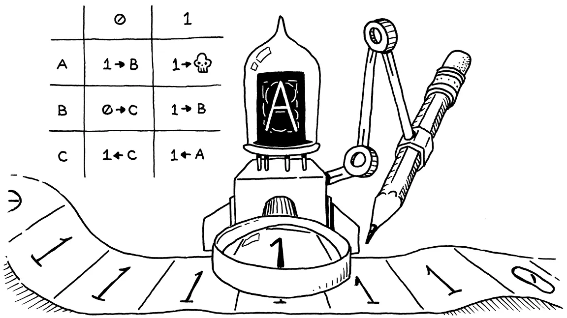
First off, what are P and NP? They are sets of decisions problems defined by how long it takes a (non-)deterministic turing machine to solve them. P is the set of decision problems which can be solved in polynomial time using a turing machine. NP is the set of all problems which can be solved in polynomial time using a non-deterministinic turing machine. We elaborate more on turing machines in a bit. But for now, just think it as a machine loaded with a program which has a tape of symbols which it can read, write, and jump around on.

Decision Problems

A decision problem is a yes-no question and it evaluates to true or false: deciding if \(\sqrt{2}\) is a rational number is a decision problem. Decision problems are fundementally different than counting problems which ask how many of something there is. For instance, given a rook at a1 on chess board, how many ways can it get h8 without crossing the main diagonal?

Formally, we can define a decison problem as follows. Given a finite (set) alphabet \(\Sigma\), the set of all finite strings generated from over the alphabet is \(\Sigma^*\) and \(L \subseteq \Sigma^*\) is some subset of strings. We say \(L\) is decidable iff there is an algorithm, \(M\) (e.g turing machine), which correctly accepts or rejects all strings in \(\Sigma^*\) (i.e \(\forall x \in \Sigma^*\) \(M(x)\) terminates and \(M(x) =\) accept iff \(x \in L\)).

Turing Machines

Formally, a deterministic turing machine is has:

• \(K\): a finite set of states
• \(\Sigma\): a finite alphabet
• \(s\): an initial state
• \(\delta : (K \times \Sigma) \to K \cup \{acc, rej\} \times \Sigma \times \{L,S,R\}\): a transition function which takes as input the current state and symbol on the tape and then updates the state, writes (possible the same) symbol to the tape or terminates with an accept or reject. If the program hasn’t terminated, the machine also a step to the left or right along the tape, or remains stationary.

A turing machine repeatedly applies the transition function, updating its current state and editing the tape. This process repeats forever or until the turing machine reaches a terminal state. Side note: deciding whether a turing machine will terminate for a given initialization is known as the halting problem and is undecidable in general.

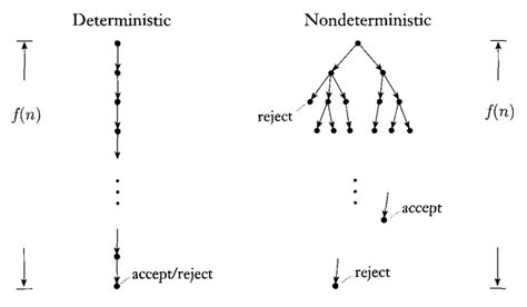
The only difference between a deterministic turing machine and a non-deterministic turing machine is that transition function is generalized to an arbitrary relation: \(\delta \subseteq (K \times \Sigma) \times (K \cup \{acc, rej\} \times \Sigma \times \{L,S,R\})\). In other words, each state and symbol can transition into multiple possible states. The power of non-determinism is that we can explore multiple branches of computation at once. A string \(x\) is accepted it at least on the branches produces an accept.

Two definitions for NP

For a determinstic turing machine, the runtime is completely determined by current state \(q\), the tape upto and including the turing machine’s current positiuon \(w\), and the remaining tape \(u\). We call \((q, w, u)\) the configution and at the step the turing machine yields a new configuration according to the rules of the transition function:

\[(q, w, u) \to_M (q', w', u')\]

Define \(\to^*_M\) as the transitive and reflective closure of \(\to_M\). In other words, for a is a sequence of configurations \(c_1...c_n\) where \(c_i \to_M c_{i+1}\), then \(c_i \to^*_M c_j\) for all pairs \(i, j\) where \(i \leq j\). We call \(c_1...c_n\) a computation of \(M\).

The language accepted by a turing machine \(L(M) \subseteq \Sigma^*\) is the set of strings:

\[L(M) := \{x|(s,\triangleright, x) \to^*_M (acc,w,u) \space \text{for some} \space w, u\}\]

For non-deteministic turing machines, the we define \(L(M)\) identically, although it’s important to note that \(\to_M\) and \(\to^*_M\) are no longer functional relationships.

Nondeterministic Complexity

For a function \(f: \mathbb{N} \to \mathbb{N}\), we say a language \(L\) is in \(NTIME(f(n))\) if there is a non-deterministic turing machine M, such that:

• \(L\) = \(L(M)\)
• \(\forall x \in L\) there is some accepting computation \(c_1...c_n\) such that \(n < O(f(\\|x\\|))\).

The last statement is a bit of a mouth-full, so we’ll just say “the running time of \(M\) is in \(O(f\\|x\\|)\)”. We now have all the tools we need to define NP:

\[NP := \bigcup_{k=1}^{\infty}NTIME(n^k)\]

We can define \(P\) and \(TIME(f(n))\) for deterministic turing machines similarily.

Succinct Certificates

Equivalenty, NP is the collect of languages \(L\) such that:

\[L = \{x | \exists y R(x,y)\}\]

where \(R\) is a relation on strings that is 1) decidable in polynomial time and 2) polynomially balanced: there is a polynomial \(p\) such that if \(R(x,y)\) and the length \(x\) is \(n\), then the length of \(y\) is no more than \(p(n)\).

We’ll now show these definitions are equaivalent. Consider a language \(L = \{x \\| \exists y R(x,y)\}\). Using a non-deterministic machine M, we can use branching to guess at values for \(y\). Because \(R\) is polynomially-balanced, then there will be a computation polynominal in \(n=\\|x\\|\).

Now suppose we are given a non-deterministic turing machine \(M\) which runs in time \(p(n)\). Because \(K\) and \(\Sigma\) are finite then there is some bound \(k\) for each state and symbol pair \((q, \sigma)\), \(\delta(q, \sigma)\) has at most \(k\) elements. Consider a string \(y\) over an alphabet \(\{1...k\}\). We define the relation \(R(x,y)\) by:

• \(\\|y\\| < p(\\|x\\|)\),
• The computation of \(M\) on \(x\) which at step \(i\) takes the \(y[i]\)th transition is an accepting computation

In other words, we can enumerate all possible computations \(x \in L\) with strings \(y\). Then by construction, \(R(x,y)\) iff there is an accepting computation of \(M\) of \(x\). What this means is that the language \(L' = \{x \\| \exists y R(x,y)\}\) is equivalent to \(L\). Done.

Simply put, \(y\) represents any sequence of computations with length \(< p(\\|x\\|)\). If \(R(x,y)\) then \(M(x)\) must accept \(x\). Referring to the image above, \(y\) is just an accepting branch of computation. It’s not too hard to see that we could construct a determinstic machine which takes in \(x\) and \(y\) as input and and can verify that \(R(x,y)\). This what is meant by saying that problems in NP are hard to solve but easy to verify: the lengths of their cerificates are polynomial so their verification can be done in P.